Restaurants, Rats, and 311 Complaints: Mapping NYC’s Rodent Hotspots
Author
WingChan
Introduction
New York City is a global dining hub, with restaurants seemingly on every street corner. At the same time, the city is infamous for rodent sightings, often reported through 311 complaints. The COVID-19 pandemic reshaped the city’s dining landscape: indoor dining was temporarily halted, and the Open Restaurants Program was launched, enabling restaurants to apply for outdoor seating.
Given this unique intersection of dense restaurant activity, expanded outdoor dining, and persistent rodent issues, it is important to understand how these factors may be related. This analysis aims to uncover patterns and insights connecting restaurant density, outdoor seating, and rodent complaints across the city focusing on the following key areas:
Neighborhoods with elevated density of rodent-related restaurant inspections
Temporal and spatial trends in rodent complaints
Potential influence of outdoor dining on rodent complaints
Correlation between restaurant-related rodent activity and 311 complaints
Datasets used:
DOHMH Restaurant Inspections (2024–2025, including rodent-related violations)
This dataset provides the data tracks all violations, scores, and grades from inspections of NYC restaurants.
The following process loaded the raw data and then filtered it to capture only the most recent, relevant inspection for each restaurant. This was achieved by selecting specific inspection types (like cycle or re-inspection) and records with a passing score or an assigned grade, ensuring the focus is solely on the current, final status of each establishment.
Code
library(readr)library(tidyverse)# Download DOHMH NYC Restaurant Inspection Results data set and save as CSV file: NYC_Insp_Results.csvOpen_Data_Sample <-read_csv("data/project/DOHMH_New_York_City_Restaurant_Inspection_Results_20251105.csv",col_types=cols(ZIPCODE =col_character()))#Filter on inspection type, score, gradeInspections <- Open_Data_Sample %>%filter((`INSPECTION TYPE`%in%c('Cycle Inspection / Re-inspection' ,'Pre-permit (Operational) / Re-inspection')|(`INSPECTION TYPE`%in%c('Cycle Inspection / Initial Inspection' ,'Pre-permit (Operational) / Initial Inspection')) & SCORE <=13)| (`INSPECTION TYPE`%in%c('Pre-permit (Operational) / Reopening Inspection' ,'Cycle Inspection / Reopening Inspection'))& GRADE %in%c('A', 'B', 'C', 'P', 'Z')) %>%select(CAMIS,`INSPECTION DATE`)#Select distinct inspectionsInspections_Distinct <-distinct(Inspections)#Select most recent inspection dateMostRecentInsp <- Inspections_Distinct %>%group_by(CAMIS) %>%slice(which.max(as.Date(`INSPECTION DATE`,'%m/%d/%Y')))#Join most recent inspection with original datasetinner_join(Open_Data_Sample,MostRecentInsp, by ="CAMIS","INSPECTION DATE")#Select restaurant inspection data based on most recent inspection dateFinal <- Open_Data_Sample %>%inner_join(MostRecentInsp) %>%filter((`INSPECTION TYPE`%in%c('Cycle Inspection / Re-inspection' ,'Pre-permit (Operational) / Re-inspection' , 'Pre-permit (Operational) / Reopening Inspection' ,'Cycle Inspection / Reopening Inspection')|(`INSPECTION TYPE`%in%c('Cycle Inspection / Initial Inspection' ,'Pre-permit (Operational) / Initial Inspection')) & SCORE <=13)) %>%select(CAMIS,DBA,`INSPECTION DATE`,GRADE,`INSPECTION TYPE`,`VIOLATION CODE`, `VIOLATION DESCRIPTION`,`CRITICAL FLAG` ,BORO, BUILDING,STREET,ZIPCODE, NTA,Latitude,Longitude) #select necessary columns# filter(`VIOLATION CODE` %in% c("08A", "04K", "04L"))%>% #Filter the violation with mice, rat, rodent related inspection, assuming those are rest with rodent issue###Select distinct restaurant inspection dataFinal <-distinct(Final)glimpse(Final) Final <- Final %>%mutate(`INSPECTION_DATE`=mdy(`INSPECTION DATE`))Final %>%arrange(`INSPECTION_DATE`)Final|>arrange(desc(`INSPECTION_DATE`))Final <- Final %>%filter(year(INSPECTION_DATE) %in%c(2024, 2025))glimpse(Final)
The data tracks all rodent-related problems reported by NYC residents to the 311 service line, covering complaints about rats, mice, or sanitation issues. It records the exact date, time, and location of the problem, along with the subsequent action taken by the Department of Health.
The following acquisition process pull the data directly from the city’s open data source via API. The function is written to download the data responsibly. It page through the entire data set with repeated requests to the server, downloading the entire history of complaints in small batches, one after the other. All these individual batches were then combined into one final dataset for analysis. It is also designed to adopt a strategy of caching results.
Code
library(httr2) library(jsonlite) library(dplyr) library(sf) library(purrr) library(tidyr)# This makes the workflow reproducible and avoids re-downloading each time. # Since we are not creating any docs or files right now, this is for later reference. if (!dir.exists("data/final")) { dir.create("data/final", showWarnings =FALSE, recursive =TRUE) } # Function to download 311 rat complaints ##################################################### # Define file pathrat311_file <-"data/final/rat311_full.rds"get_rat311_full <-function() { base_url <-"https://data.cityofnewyork.us/resource/cvf2-zn8s.geojson" limit <-50000# max per request offset <-0 all_data <-list()repeat { resp <-request(base_url) %>%req_url_query("$limit"= limit,"$offset"= offset ) %>%req_perform()resp_check_status(resp) raw_json <-resp_body_string(resp) gj <-fromJSON(raw_json, flatten =TRUE)# Convert features to tibble dat <- gj$features %>%as_tibble()if (nrow(dat) ==0) break# stop if no more rows all_data[[length(all_data) +1]] <- dat offset <- offset +nrow(dat)cat("Downloaded rows:", offset, "\n") }# Combine all pages into a single tibblebind_rows(all_data)}# Check if file exists, otherwise downloadif (file.exists(rat311_file)) { rat311_full <-readRDS(rat311_file)cat("Loaded rat 311 data from local file.\n")} else { rat311_full <-get_rat311_full()saveRDS(rat311_full, rat311_file)cat("Downloaded rat 311 data and saved locally.\n")}# Quick look at the dataglimpse(rat311_full)
This dataset tracks all historical applications submitted by New York City restaurants to participate in the Open Restaurant Program, which permits temporary expansion of seating onto sidewalks and roadways during COVID period. The temporary emergency program was ended in Aug 2023, replaced by the permanent “Dining Out NYC” initiative.
The following acquisition process involved reading a file containing the complete application history, and the accompanying code then filtered this history to keep only the most recent application for each unique restaurant. This step ensures that the final data used for analysis accurately reflects once for every establishment that applied to the program.
Code
open_rest <-read_csv("data/project/Open_Restaurant_Applications_(Historic)_20251107.csv")glimpse(open_rest)summary(open_rest)open_rest <- open_rest %>%mutate(`SubmissionDateTime`=mdy_hms(`Time of Submission`))open_rest %>%arrange(`SubmissionDateTime`) |>select(SubmissionDateTime)#get distinct resturant applicationdistinct_open_rest <- open_rest |>group_by(`Food Service Establishment Permit #`) %>%arrange(desc(`Time of Submission`), .by_group =TRUE) %>%slice_head(n =1) %>%ungroup()
The data provides the official geographic boundaries (shapes) for all Neighborhood Tabulation Areas (NTAs) across New York City, which are standardized, mid-sized statistical units used by the Department of City Planning. It is essential for geographically linking the data (inspections, complaints, and open resturants) to a neighborhood level for analysis.
The acquisition process involved using a computer script to retrieve the required GeoJSON file (a type of geographic data format) from the city’s server. To maintain efficiency, the script was designed to download and save the file only once locally, after which it reads the data and prepares the map by setting all coordinates to the standard Latitude/Longitude system, making it immediately ready for geographic analysis with other datasets.
Code
# Downloads and prepares NTA polygons ###################################### # This URL serves the 2020 NTA boundaries as a (projected) GeoJSON from ArcGIS. nta_url <-"https://services5.arcgis.com/GfwWNkhOj9bNBqoJ/arcgis/rest/services/NYC_Neighborhood_Tabulation_Areas_2020/FeatureServer/0/query?where=1=1&outFields=*&outSR=4326&f=pgeojson"nta_path <-"data/final/nta_2020.geojson"# To keep the workflow efficient and reproducible, this: # - Downloads the file once and saves it locally # - Reuses the local file in future runs instead of hitting the server again if (!file.exists(nta_path)) { resp <-request(nta_url) |>req_perform() resp_check_status(resp) resp_body_raw(resp) |>writeBin(con = nta_path) } # Reads the saved NTA GeoJSON as an sf object (polygons). # st_transform(4326) ensures everything is in WGS84 lat/lon (EPSG:4326), # which matches the coordinates used in the rat 311 data. nta <-st_read(nta_path, quiet =TRUE) |>st_transform(4326) glimpse(nta)
Data Integration & Exploration
Neighborhoods with elevated density of rodent-related restaurant inspections
This section will perform an initial assessment of the restaurant inspection data to identify which New York City neighborhoods (NTAs) face the highest concentration of rodent-related issues.
The analysis first determines the total number of inspections and the percentage of those inspections that resulted in a rodent-related violation. We then identify and categorize these violations based on their severity (Critical vs. Not Critical). Finally, we calculate the density of rodent violations per unit of neighborhood area to fairly compare neighborhoods of different sizes, pinpointing the top ten NTAs with the most elevated rodent-related restaurant inspection activity. The results will be visualized using a geospatial map to illustrate where these high-density areas are located across the city.
Integrate DOHMHInspection data with NTA
To prepare the inspection records for neighborhood-level analysis, this code first takes the restaurant inspection data’s coordinates and converts them into mappable points. Then, it performs a spatial join to attach the corresponding Neighborhood Tabulation Area (NTA) code and name to each inspection record. This is necessary because the original inspection data only contains exact street coordinates, but our analysis requires us to group and compare restaurant issues at the neighborhood (NTA) level.
Code
# Converts inspection coordinates into sf points ########################################## DOHMHInspection <- Final |>mutate( lon =as.numeric(Longitude), lat =as.numeric(Latitude) ) |>drop_na(lon, lat)DOHMHInspection_sf <- DOHMHInspection %>%st_as_sf(coords =c("lon", "lat"), crs =4326,remove =FALSE )#spatial join to look up NTA DOHMHInspection_NTA <-st_join( DOHMHInspection_sf, nta[, c("NTA2020", "NTAName", "BoroName","Shape__Area")] # <- adjust to actual column names ) glimpse(DOHMHInspection_NTA)
DOHMH New York City Restaurant Inspection Exploration
This step is to examine the overall inspection data to understand the most common issues and isolate rodent-related cases.
Code
# Drop this geometry for analyticsDOHMHInspection_NTA_clean <-st_drop_geometry(DOHMHInspection_NTA)# Check data periodperiod_DOHMHInspection <- DOHMHInspection_NTA_clean %>%select(-NTA)%>%mutate(`INSPECTION DATE`=mdy(`INSPECTION DATE`)) %>%# convert to Datesummarise(min_date =min(`INSPECTION DATE`, na.rm =TRUE),max_date =max(`INSPECTION DATE`, na.rm =TRUE) )# Total # of Inspectiontot_inspection <-nrow(DOHMHInspection_NTA_clean)# What are the issue found from the inspection?violation_summary <- DOHMHInspection_NTA_clean %>%group_by(`VIOLATION CODE`, `VIOLATION DESCRIPTION`) %>%summarise(count =n(), .groups ="drop") %>%mutate(percent_of_total = count /sum(count) *100) %>%arrange(desc(count))# What are mice, rat, rodent related case?DOHMHInspection_NTA_rodent <- DOHMHInspection_NTA_clean %>%filter(`VIOLATION CODE`%in%c("08A", "04K", "04L"))rodent_insepction <- DOHMHInspection_NTA_rodent %>%nrow()percent_rodent <- rodent_insepction / tot_inspection *100# Out of the rodent case from the inspection how many are critical || Rodent case summaryrodent_summary <- DOHMHInspection_NTA_rodent %>%group_by(`CRITICAL FLAG`, `VIOLATION CODE`, `VIOLATION DESCRIPTION` ) %>%summarise(count =n(), .groups ="drop") %>%mutate(percent = count /sum(count) *100) %>%arrange(desc(count))# Where are the neighborhood with most rat inspection case? # For Critical cases DOHMHInspection_NTA_rodent_critical <- DOHMHInspection_NTA_rodent %>%filter(`VIOLATION CODE`%in%c("04K", "04L"))Top_DOHMHInspection_NTA_rodent_critical <- DOHMHInspection_NTA_rodent_critical %>%group_by(NTA2020, NTAName) %>%summarise(total_inspections =n()) %>%arrange(desc(total_inspections)) %>%head(10) # Top 10 NTA# For Not Cirtical CasesDOHMHInspection_NTA_rodent_critical <- DOHMHInspection_NTA_rodent %>%filter(`VIOLATION CODE`%in%c("08A"))Top_DOHMHInspection_NTA_rodent_not_critical <-DOHMHInspection_NTA_rodent_critical %>%group_by(NTA2020, NTAName) %>%summarise(total_inspections =n()) %>%arrange(desc(total_inspections)) %>%head(10) # Top 10 NTA
Key finding
Total Inspections: 59020 inspections were performed during the analyzed period (2024-01-02 to 2025-11-01).
Rodent Prevalence: Violations related to rats, mice, or rodents constituted 12.87% of the total inspections. These violations are among the most common issues flagged, with Violation Code 08A being the 3rd most frequent overall, and 04L being the 8th most frequent overall.
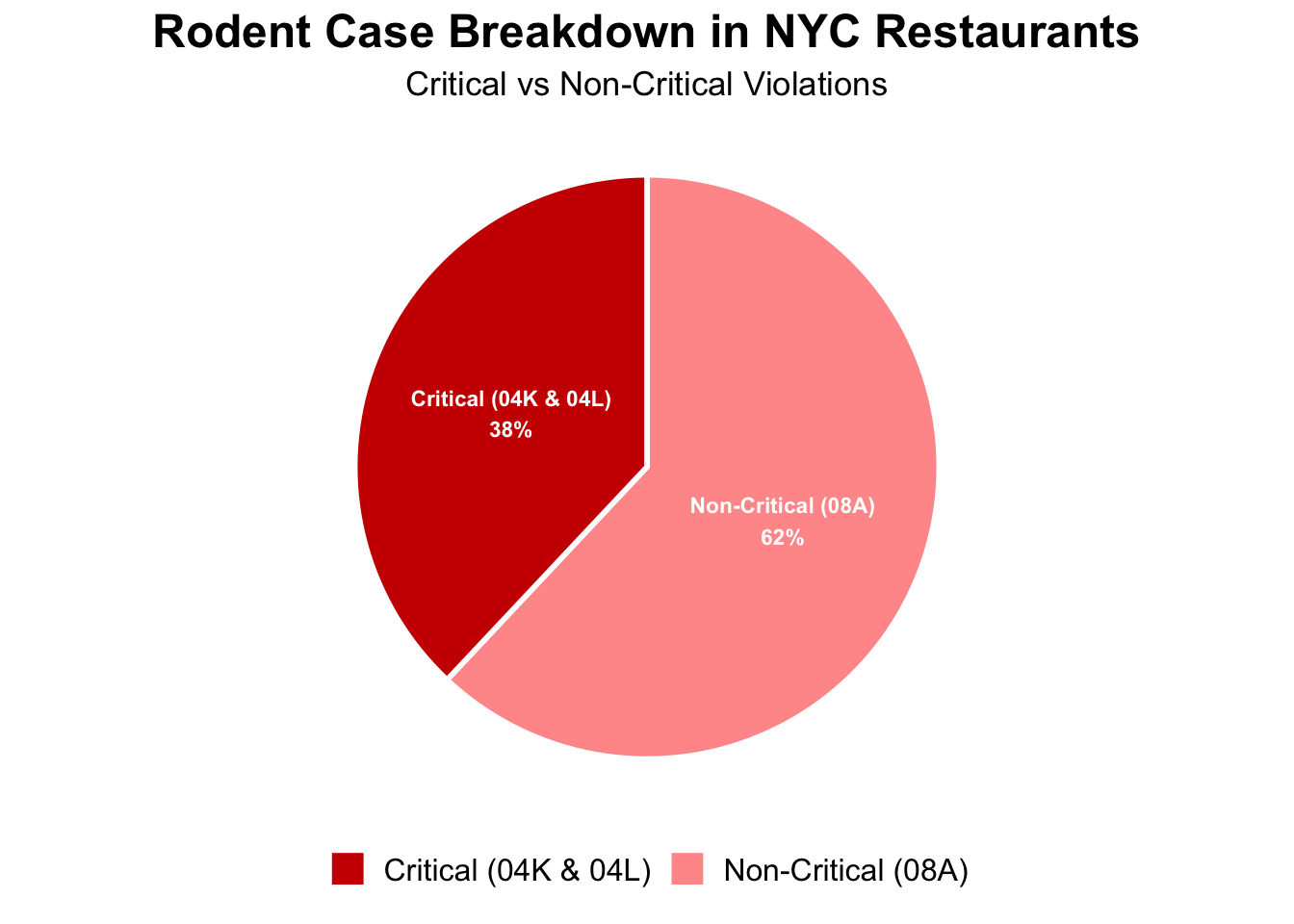
Rodent Case Breakdown:Not Critical (08A): 62% of rodent-related cases fell under the non-critical category, citing conditions that allow pests like rodents and insects to thrive.Critical (04K & 04L): 38% of cases were critical violations, citing evidence of mice or live mice in the establishment’s food or non-food areas.
Code
library(ggplot2)library(dplyr)# Create the datarodent_data <-data.frame(Category =c("Non-Critical (08A)", "Critical (04K & 04L)"),Percentage =c(62, 38),Label =c("Non-Critical (08A)\n62%", "Critical (04K & 04L)\n38%"),Description =c("Conditions that allow pests\n(rodents/insects) to thrive","Evidence of mice or live mice\nin food/non-food areas"))# Pie chartggplot(rodent_data, aes(x ="", y = Percentage, fill = Category)) +geom_bar(stat ="identity", width =0.5, color ="white", size =1) +coord_polar(theta ="y") +geom_text(aes(label = Label),position =position_stack(vjust =0.5),size =3, fontface ="bold", color ="white") +scale_fill_manual(values =c("Non-Critical (08A)"="#FF9999", "Critical (04K & 04L)"="#CC0000")) +labs(title ="Rodent Case Breakdown in NYC Restaurants",subtitle ="Critical vs Non-Critical Violations",caption ="Source: NYC DOHMH Restaurant Inspections") +theme_void() +theme(plot.title =element_text(size =18, face ="bold", hjust =0.5),plot.subtitle =element_text(size =13, hjust =0.5),legend.position ="bottom",legend.title =element_blank(),legend.text =element_text(size =12),plot.caption =element_text(size =8, color ="white") ) +guides(fill =guide_legend(override.aes =list(color ="white")))
Normalization and High-Density Neighborhoods
To fairly compare areas of different sizes, the analysis then calculated the rodent-related inspection density by normalizing the rodent case count by the neighborhood’s area (cases per 10,000 units of area).
Code
## Normalizing by calcualte the rodent restaruant / area helps compare neighborhoods of different sizes fairly.## Density is calculated as #case per 10,000 Units of Arearodent_density <- DOHMHInspection_NTA_rodent %>%group_by(NTA2020, NTAName, Shape__Area) %>%summarise(rodent_count =n(), .groups ="drop") %>%mutate(density_per_10000_area =round((rodent_count / Shape__Area) *10000, 2)) rodent_density_top10 <- rodent_density%>%select (-Shape__Area)%>%arrange(desc(density_per_10000_area)) %>%head(10) # Top 10 NTA
Key finding
The results clearly indicate a significant clustering of high-density rodent activity in Manhattan. Midtown and Lower Manhattan neighborhoods dominate the list when normalizing for land area.
Using a interactive geospatial visualization to map the rodent violation density across all Neighborhood Tabulation Areas (NTAs), visually confirming the areas of highest risk.
The geospatial map confirms that the highest concentrations (darkest red) of rodent-related restaurant inspection activity are overwhelmingly located in the denser commercial and residential areas of Manhattan and inner Brooklyn.
Temporal and Spatial Trends in Rodent Complaints Align with Restaurant Inspection Period
This section conducts an initial analysis of 311 Rodent Complaints within the same timeframe as the restaurant inspections (January 2, 2024, to November 1, 2025) to identify which neighborhoods report the highest volume of rodent activity.
The analysis first determines the total number of complaints recorded during the period, followed by a time-series plot to visualize the monthly trend of complaints. We then calculate the raw count of complaints per Neighborhood Tabulation Area (NTA) to see where the highest numbers are reported. Finally, to ensure a fair comparison across neighborhoods of varying sizes, we calculate the complaint density per unit of neighborhood area, pinpointing the top ten NTAs with the most concentrated rodent complaint activity for comparison with the restaurant inspection findings.
Integrate 311 Rodent Complaints data with NTA
The 311 Rodent Complaints data is integrate with the Neighborhood Tabulation Areas (NTAs) as a preparation for the analysis. This is a crucial step because the original complaint data only provides coordinates, but our analysis requires grouping and comparing the frequency of these issues at the standardized neighborhood (NTA) level.
The code first prepares the raw complaint records by extracting the latitude and longitude and converting the data into mappable points. Then, a spatial join is then executed, which effectively assigns the corresponding NTA code, name, and area to each complaint based on where the point falls on the map.
Code
#1a. Rat complaints + NTA# Converts rat coordinates into sf points ########################################## # Rat points# The 311 data stores coordinates inside the properties fields. # The following: # - Extracts longitude and latitude as numeric columns # - Drops any rows where coordinates are missing rat_coords <- rat311_full |>mutate( lon =as.numeric(properties.longitude), lat =as.numeric(properties.latitude) ) |>drop_na(lon, lat) # Converts the rat complaints from a regular tibble to an sf object with POINT geometry. # This is necessary so we can do spatial operations like joins with NTA polygons. rats_sf <-st_as_sf( rat_coords, coords =c("lon", "lat"), crs =4326) # Spatial join to assign each rat point to an NTA ################################################## # Keeps only the NTA identifier/name/borough columns for the join to keep it light. # st_join() will assign to each rat point the attributes of the polygon it falls inside. rats_with_nta <-st_join( rats_sf, nta[, c("NTA2020", "NTAName", "BoroName", "Shape__Area")] # <- adjust to actual column names ) # Drop geometry for a regular tabular data frame ################################################ # After we’ve done the spatial join, we may want to work with the data # as a regular tibble (to joins to other tables or other analysis). # st_drop_geometry() removes the geometry column but keeps the NTA info. rats_with_nta_df <- rats_with_nta |>st_drop_geometry() # Final sanity check: view the resulting columns. # At this stage, you should see original rat 311 fields + NTA2020, NTAName, BoroName. glimpse(rats_with_nta_df)
311 Rodent Complaint Data Exploration and Time-Series Analysis
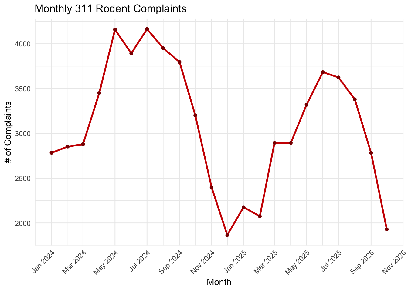
This step filters the 311 Rodent Complaints to match the time frame of the restaurant inspections (Jan 2024 to Nov 2025), establishing a consistent period for analysis. It then calculates the total number of complaints and aggregates them by month to produce a line chart showing the complaint trend over time. This visual helps monitor seasonal or continuous changes in reporting activity.
Code
library(dplyr)library(lubridate)rat311_filtered_2024 <- rats_with_nta_df %>%mutate(created_date =ymd_hms(properties.created_date) # Convert the character string to a POSIXct (datetime) object ) %>%filter(created_date >=as.Date("2024-01-02") &#filter period that align with restaraunt inspection created_date <=as.Date("2025-11-01"))#total number of complaintstot_rat_complaints <-nrow(rat311_filtered_2024)rat311_filtered_month <- rat311_filtered_2024 %>%mutate(year_month =floor_date(created_date, "month")) %>%group_by(year_month) %>%summarise(complaint_count =n(), .groups ="drop")%>%mutate(year_month =as.Date(year_month))ggplot(rat311_filtered_month, aes(x = year_month, y = complaint_count)) +geom_line(color ="red3", size =1) +geom_point(color ="darkred") +scale_x_date(date_labels ="%b %Y", date_breaks ="2 months") +labs(title ="Monthly 311 Rodent Complaints",x ="Month",y ="# of Complaints" ) +theme_minimal() +theme(axis.text.x =element_text(angle =45, hjust =1))
Key finding
Based on the analysis of 68160 311 Rodent Complaints filed between January 2, 2024, and November 1, 2025.
The rodent complaints demonstrate a strong seasonal pattern, generally starting to rise in April and peaking during the warmer summer months (May–July) before dropping off around October. This cyclical pattern appeared consistent between 2024 and 2025.
Raw Complaint Count by Neighborhood
Code
### Where are the neighborhood with highest # of complaints? # Count complaints per NTArat311_by_nta <- rat311_filtered_2024 %>%group_by(NTAName, NTA2020) %>%summarise(complaint_count =n(), .groups ="drop") %>%arrange(desc(complaint_count))# View top neighborhoodstop_rat311_by_nta <-head(rat311_by_nta, 10)
Key Finding - The top-ranking neighborhoods concentrated in Upper Manhattan and specific dense areas of the Bronx and also in Brooklyn and Queens.
To fairly compare areas, the data was normalized by neighborhood area (density). The density calculation reveals neighborhoods where the problem is most concentrated.
Code
#which NTA has highest density of rodent problem reportedrat311_density <- rat311_filtered_2024 %>%group_by(NTA2020, NTAName,Shape__Area) %>%summarise(complaint_count =n(), .groups ="drop") %>%mutate(density_per_10000_area = complaint_count / Shape__Area *10000 ) %>%arrange(desc(density_per_10000_area))# View top 10 NTAs by densitytop_rat311_density <-head(rat311_density, 10) |>select (NTAName, NTA2020, density_per_10000_area)
Both the raw count and the density ranking (complaints per 10,000 units of area) highlighted neighborhoods in Upper Manhattan (like Central and East Harlem), Brooklyn, and Queens as areas with the highest reported issues.
Comparing with Restaurant Inspection Findings, the geographic pattern of 311 complaints differs significantly from the location of high-density rodent violations found in restaurant inspections.
The highest density of rodent-related restaurant violations was primarily concentrated in Mid-Manhattan’s central business districts (e.g., Midtown South, East Village, Lower East Side), reflecting commercial activity.
Conversely, the highest density of 311 public complaints is focused in Upper Manhattan (Harlem) and surrounding boroughs, suggesting that the public perceives the rodent problem as more concentrated in these residential and mixed-use areas.
Potential influence of outdoor dining on rodent complaints
This analysis utilizes the NYC Open Restaurants Program dataset, introduced in June 2020 to facilitate outdoor dining when indoor seating was restricted due to COVID-19. As this data provides a longer timeline than the one-year DOHMHInspection data, it serves as a supplement for exploring the temporal and spatial connections between the proliferation of outdoor seating (and potential sanitary risks) and the rise in rodent complaints.
The analysis first analysis the total number of Open Restaurant applications submitted between June 2020 and August 2023 and visualizes the application trend over time. We then calculate the density of Open Restaurant applications per unit of neighborhood area to pinpoint the top ten NTAs where outdoor seating proliferation was most concentrated. Finally, the analysis filters 311 Rodent Complaints to the same time period and calculates the density of these complaints in each NTA, allowing for a direct comparison of the geospatial relationship between outdoor dining density and reported rodent issues across the city.
Integrate 311 Rodent Complaints data with NTA
The Open Restaurant application data is integrated with the Neighborhood Tabulation Areas (NTAs) as a preparation for spatial analysis. Although the original dataset provided the NTA name, it lacked the standardized NTA code and area information necessary for density calculations and alignment with other analyses.
The below code first prepares the raw application records by extracting the latitude and longitude and converting the data into mappable points. A spatial join is then executed, which uses these coordinates to accurately assign the corresponding standardized NTA code, name, and area (Shape__Area) to each application. It enables us to group the applications and reliably calculate the density of outdoor seating at the required neighborhood level.
Code
#4a. OpenResturant + NTA# Converts OpenResturant coordinates into sf points ########################################## open_rest <- open_rest |>mutate( lon =as.numeric(Longitude), lat =as.numeric(Latitude) ) |>drop_na(lon, lat)open_rest_sf <- open_rest %>%st_as_sf(coords =c("lon", "lat"), crs =4326,remove =FALSE )open_rest_NTA <-st_join( open_rest_sf, nta[, c("NTA2020", "NTAName", "BoroName","Shape__Area")] # <- adjust to actual column names ) glimpse(open_rest_NTA)
Open Restaurant Applications (Historic) data Exploration
This step is to examine the overall Open Restaurant Applications data to understand the application trend and neighborhood with highest outdoor seating.
Code
#drop geo code for analysisopen_rest_NTA <- open_rest_NTA %>%st_drop_geometry() #Check data periodperiod_open_rest_NTA <- open_rest_NTA %>%summarise(min_date =min(as.Date(SubmissionDateTime), na.rm =TRUE),max_date =max(as.Date(SubmissionDateTime), na.rm =TRUE) )#total number of applications = no. resturants had outdoor seatingtot_openseat =nrow(open_rest_NTA)tot_openseatlibrary(dplyr)library(ggplot2)library(lubridate)# Summarize number of applications per monthmonthly_apps <- open_rest_NTA %>%mutate(submit_date =as.Date(SubmissionDateTime), # convert to datemonth =floor_date(submit_date, "month")) %>%# get first day of monthgroup_by(month) %>%summarise(n_applications =n(), .groups ="drop")#find top NTAopen_rest_NTA_top10 <- open_rest_NTA %>%group_by(NTA2020, NTAName) %>%summarise(n_applications =n(), .groups ="drop") %>%arrange(desc(n_applications)) %>%slice_head(n =10)open_rest_NTA_top10# normalize the # of outdoor seating resturant by divided by the area of NTA - to be fairdensity_outdoor_by_nta <- open_rest_NTA %>%# count applications per NTAgroup_by(NTA2020, NTAName) %>%summarise(n_applications =n(),# area is repeated per row, so take first non-NA valuenta_area =first(Shape__Area),.groups ="drop" ) %>%mutate(application_density = n_applications / nta_area ) %>%arrange(desc(application_density))density_outdoor_by_nta_top10 <-density_outdoor_by_nta %>%select(NTA2020,NTAName,application_density) %>%slice_head(n=10)
Key Findings
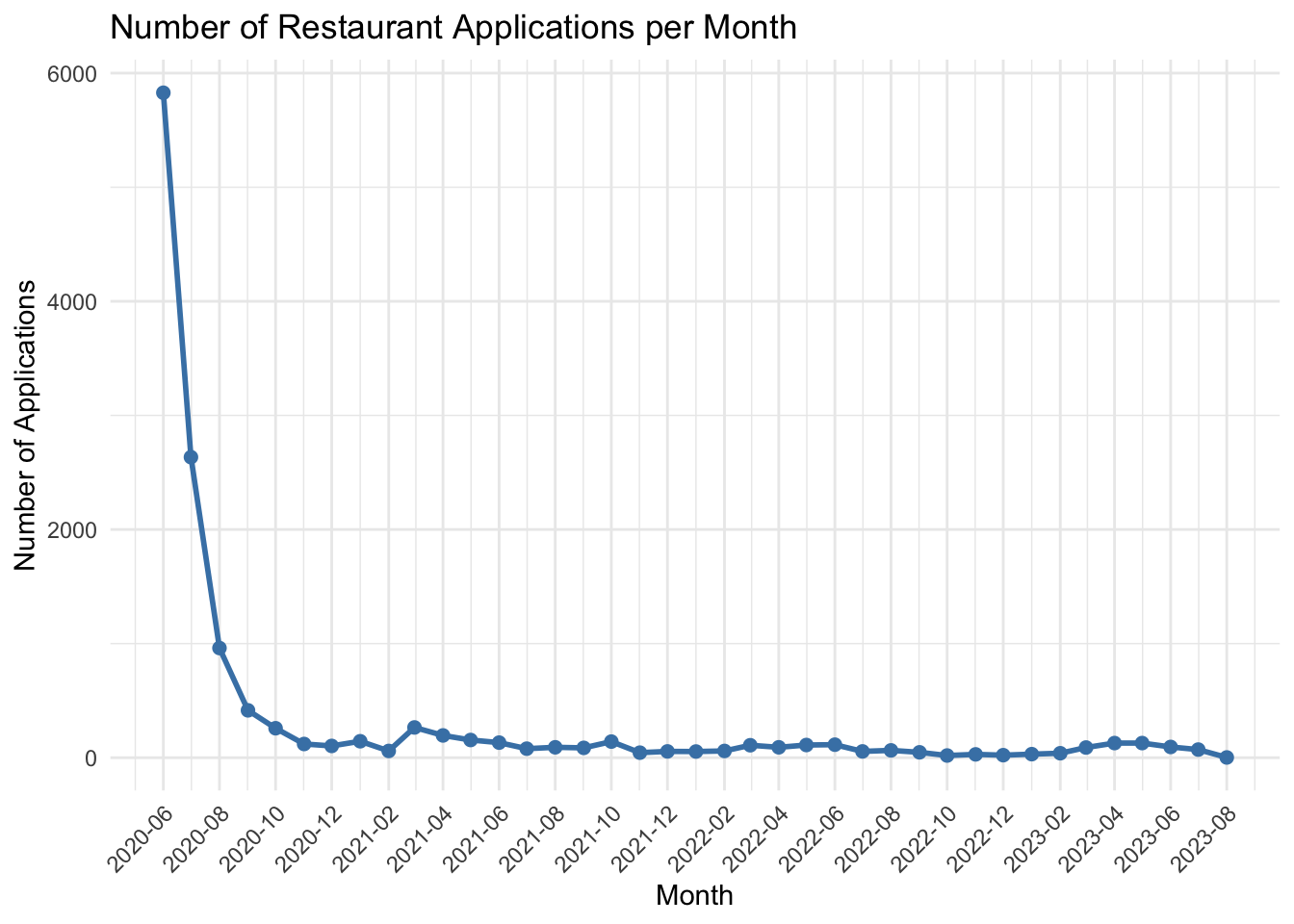
In the period of 2020-06-19 to 2023-08-02, there are 13121 number of applications.
The application volume peaked dramatically during the initial months, specifically from June to August 2020. This surge reflects the urgent need for restaurants to adapt and survive the pandemic-induced shutdown of indoor dining, with the application rate naturally slowing down significantly thereafter.
Code
# Plot line chartggplot(monthly_apps, aes(x = month, y = n_applications)) +geom_line(color ="steelblue", size =1) +geom_point(color ="steelblue", size =2) +labs(title ="Number of Restaurant Applications per Month",x ="Month",y ="Number of Applications" ) +theme_minimal() +scale_x_date(date_labels ="%Y-%m", date_breaks ="2 months") +theme(axis.text.x =element_text(angle =45, hjust =1))
the highest number of outdoor seating applications were overwhelmingly concentrated in Manhattan’s commercial and dense residential centers. Specifically, the top neighborhoods for application volume are located in Downtown and Mid-Manhattan (e.g., East Village, Midtown, West Village). Outside of Manhattan, the only two neighborhoods that made the top application list were Williamsburg and Park Slope in Brooklyn.
To ensure a fair comparison across neighborhoods of varying sizes, the density of Open Restaurant applications (applications per unit of area) was calculated. This analysis revealed that the highest concentration of outdoor seating was overwhelmingly located in Manhattan’s most commercially dense districts, specifically Downtown and Mid-Manhattan (e.g., East Village, Greenwich Village, Midtown South). This pattern highlights the intense utilization of outdoor space in the city’s central business and entertainment areas during the program period.
Temporal and spatial trends in rodent complaints Align with Open Restaurant Period
This section conducts an initial analysis of 311 Rodent Complaints filtered to the same timeframe as the Open Restaurants Program (June 19, 2020, to August 2, 2023).
The analysis first converts the date string to datetime, determines the total complaint count, and generates a time-series plot to visualize the monthly trend of complaints. We then calculate the raw count of complaints per Neighborhood Tabulation Area (NTA). Finally, to ensure fair comparison, we calculate the complaint density per unit of neighborhood area, pinpointing the top ten NTAs with the most concentrated rodent activity for direct comparison with the outdoor dining density findings.
Code
#filter the date period align with Open restaurant application datarat311_filtered_outdoor <- rats_with_nta_df %>%mutate(created_date =ymd_hms(properties.created_date) ) %>%filter(created_date >=as.Date("2020-06-19") & created_date <=as.Date("2023-08-02"))#total number of complaintstot_rat_complaints <-nrow(rat311_filtered_outdoor)### Where are the neighborhood with highest # of complaints? # Count complaints per NTArat311_outdoor_by_nta <- rat311_filtered_outdoor %>%group_by(NTAName, NTA2020) %>%summarise(complaint_count =n(), .groups ="drop") %>%arrange(desc(complaint_count))# View top neighborhoodstop_rat311_outdoor_by_nta <-head(rat311_outdoor_by_nta, 10)#which NTA has highest density of rodent problem reportedrat311_outdoor_density <- rat311_filtered_outdoor %>%group_by(NTA2020, NTAName,Shape__Area) %>%summarise(complaint_count =n(), .groups ="drop") %>%mutate(density_per_10000_area = complaint_count / Shape__Area *10000 ) %>%arrange(desc(density_per_10000_area))# View top 10 NTAs by densitytop_rat311_outdoor_density <-head(rat311_outdoor_density, 10) %>%select (NTA2020, NTAName, density_per_10000_area)
Key Findings
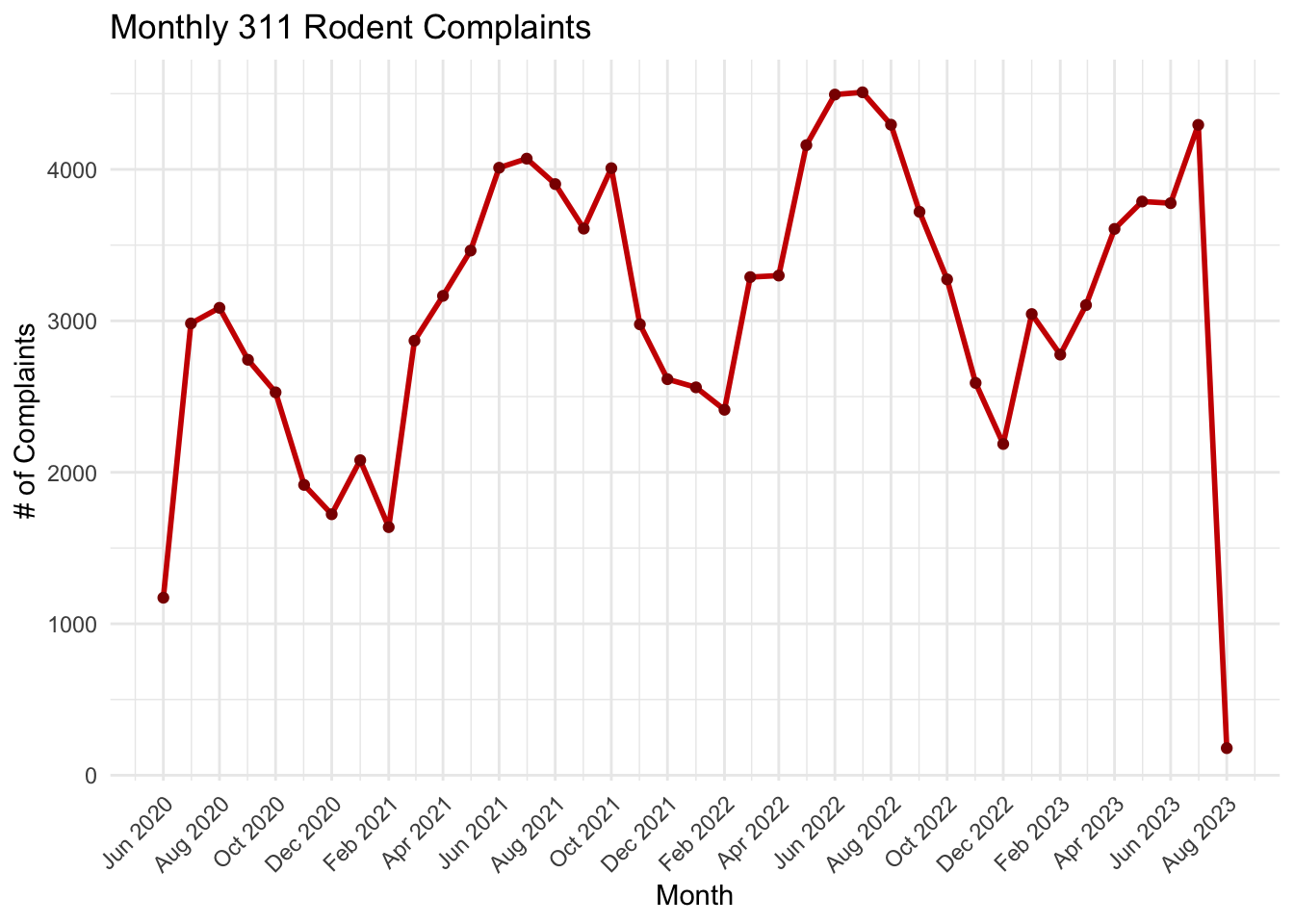
In the period of 2020-06-19 to 2023-08-02, there are total 119924 of rodent complaints
The rodent complaints demonstrate a strong seasonal pattern, generally starting to rise in April and peaking during the warmer summer months (May–July) before dropping off around October. This cyclical pattern appeared consistent between 2020 to 2023, also matching the previous analysis [here].
Based on the raw count of 311 Rodent Complaints, the highest volume of reported activity is concentrated in Brooklyn (Bedford-Stuyvesant and Crown Heights) and Upper Manhattan (Harlem and East Harlem), indicating the greatest overall burden in these dense, mixed-use areas.
The analysis of the normalized data (complaints per 10,000 units of area) shows that the most concentrated rodent problems during the Open Restaurants period (June 2020–August 2023) were found overwhelmingly in Manhattan
Eight of the top ten spots belong to Manhattan neighborhoods, specifically in Harlem (South and North), the Upper West Side, and the Upper East Side. This indicates the problem is most intense, relative to neighborhood size, in these dense residential and institutional areas.
While Brooklyn neighborhoods had the highest raw complaint counts, the density analysis shows the problem is more severe, relative to size, in Manhattan’s Upper and West Side areas.
Correlation between restaurant-related rodent activity and 311 complaints
Correlation with Restaurant inspection
This session performs a statistical analysis to understand the relationship between public perception of rodent issues and official restaurant inspection findings. The core question is whether Neighborhood (NTA) with high densities of 311 Rodent Complaints also exhibit high densities of Critical Rodent Violations in restaurants.
The process below perform a Pearson correlation to quantify the strength and direction of the linear relationship between the two normalized metrics: Rodent Complaint Density and Inspection Violation Density.
It is anticipated a positive correlation (correlation coefficient greater than 0), suggesting that areas where the public reports more rat problems tend to align with areas where inspectors find more rat problems in food establishments.
Code
#join rest inspection with 311 complaintcombined_nta <- rat311_density %>%inner_join(rodent_density, by =c("NTA2020", "NTAName"), suffix =c("_rat", "_inspection"))correlation <-cor( combined_nta$density_per_10000_area_rat, combined_nta$density_per_10000_area_inspection,method ="pearson",use ="complete.obs"# ignore rows with NA)correlation
Code
# Fit linear modellm_fit <-lm(density_per_10000_area_inspection ~ density_per_10000_area_rat, data = combined_nta)# Create prediction datapred <-data.frame(x = combined_nta$density_per_10000_area_rat,y =predict(lm_fit, newdata = combined_nta))# Make plotlibrary(ggplot2)library(plotly)p <-ggplot(combined_nta, aes(x = density_per_10000_area_rat, y = density_per_10000_area_inspection,text =paste("NTA:", NTAName,"<br>Rat Density:", round(density_per_10000_area_rat, 2),"<br>Inspection Density:", round(density_per_10000_area_inspection, 2)))) +geom_point(aes(color = density_per_10000_area_rat * density_per_10000_area_inspection), size =4, alpha =0.7) +geom_line(data = pred, aes(x = x, y = y), color ="blue", linetype ="dashed", inherit.aes =FALSE) +scale_color_gradient(low ="pink", high ="red3") +labs(x ="Rat Complaint Density (per 10k area)",y ="Restaurant Rodent Violation Density (per 10k area)",color ="Density Product",title ="Rodent Complaint vs Restaurant Inspection Density by NTA" ) +theme_minimal()ggplotly(p, tooltip ="text")
Key findings
The correlation analysis between the density of 311 Rodent Complaints and the density of Restaurant Rodent Violations yielded a Pearson correlation coefficient of 0.3085201.
The coefficient of 0.31 indicates a weak to moderate positive linear relationship between the two metrics.
This positive relationship means that neighborhoods with higher public reporting of rodent issues (311 complaints) tend to have slightly higher densities of officially recorded rodent violations in restaurants, and vice versa.
Since the correlation is not close to 1, it confirms that public perception (311 data) and official regulatory findings (inspection data) are related but are not entirely dependent.
The scatter plot visualization (implied by the correlation) likely showed several outliner neighborhoods where one density metric is significantly high while the other is low, illustrating that some areas have high public concern without high official restaurant findings, or vice versa.
Correlation with Open resturant
This session investigates the potential link between the proliferation of outdoor dining and public reports of rodent activity. The core objective is to determine if Neighborhood (NTA) with a higher density of Open Restaurant applications also saw a higher density of 311 Rodent Complaints during the same period.
The Pearson correlation is used to quantify the strength of the linear relationship between the two key normalized metrics: 311 Rodent Complaint Density and Outdoor Seating Application Density. This test helps determine if increased outdoor dining (and associated waste/seating structures) influenced the spatial pattern of rodent reports.
It is expected a positive correlation (correlation coefficient greater than 0), suggesting that areas with more concentrated outdoor dining tended to receive more rodent complaints.
Code
#join open_rest & 311 data setcombined_outdoor_nta <- rat311_outdoor_density %>%inner_join(density_outdoor_by_nta, by =c("NTA2020", "NTAName"), suffix =c("_rat", "_outdoor"))outdoor_correlation <-cor( combined_outdoor_nta$density_per_10000_area, combined_outdoor_nta$application_density,method ="pearson",use ="complete.obs"# ignore rows with NA)outdoor_correlation
Code
# Fit linear modellm_fit <-lm(application_density ~ density_per_10000_area, data = combined_outdoor_nta)# Create prediction data for the regression linepred <-data.frame(density_per_10000_area = combined_outdoor_nta$density_per_10000_area,application_density =predict(lm_fit, newdata = combined_outdoor_nta))library(ggplot2)library(plotly)p <-ggplot(combined_outdoor_nta, aes(x = density_per_10000_area,y = application_density,text =paste0("NTA: ", NTAName,"<br>Rat Density: ", round(density_per_10000_area, 4),"<br>Application Density: ", round(application_density, 6) ))) +geom_point(aes(color = density_per_10000_area * application_density),size =4, alpha =0.7) +geom_line(data = pred, aes(x = density_per_10000_area,y = application_density ),color ="blue",linetype ="dashed",inherit.aes =FALSE ) +scale_color_gradient(low ="pink", high ="red3") +labs(x ="Rat Complaint Density (per 10k area)",y ="Outdoor Seating Application Density (per 10k area)",color ="Density Product",title ="Rat Complaint Density vs Outdoor Seating Application Density by NTA" ) +theme_minimal()ggplotly(p, tooltip ="text")
Key Findings
The analysis of the relationship between 311 Rodent Complaint Density and Outdoor Seating Application Density yielded a Pearson correlation coefficient of 0.3456858.
The coefficient indicates a weak to moderate positive linear relationship between the concentration of outdoor dining and the public reporting of rodent activity.
This suggests that neighborhoods that heavily adopted the Open Restaurants Program tend to receive slightly more rodent complaints compared to neighborhoods with fewer outdoor dining spots.
The correlation is not strong (far from 1), confirming that while the presence of concentrated outdoor dining may contribute to rodent complaints (likely due to sanitation issues like increased waste), it is not the primary factor driving the overall spatial pattern of rat complaints across the city.
Comparison Point: This correlation 0.3456858 is slightly higher than the correlation found between 311 complaints and restaurant inspection violations (0.3085201) implies a shift in the factors driving public perception of rodent issues during the pandemic and Open Restaurants Program period.
The presence and concentration of outdoor dining structures is a slightly better spatial indicator of where people are filing 311 complaints than the location of officially documented, internal restaurant rodent activity.
Restaurant inspection violations primarily measure issues inside the establishment (e.g., in food storage or preparation areas). The higher correlation with outdoor seating density suggests that complaints were driven less by internal restaurant hygiene failures and more by visible, street-level issues related to the outdoor setup.
Outdoor dining areas often lead to increased refuse, improper garbage storage, and food scraps left on sidewalks or in temporary structures. These conditions create a readily available food source and shelter for rats in public view, leading directly to more sightings and complaints by residents and pedestrians.
The difference indicates that the public was reacting more strongly to the new spatial concentration of potential rat habitats and food sources on the street (outdoor dining) than to the historical pattern of documented violations inside buildings.
Conclusion: Rodent Activity, Public Perception, and the Open Restaurants Program
This analysis integrated three disparate datasets (Open Restaurant Applications, 311 Rodent Complaints, and DOHMH Inspections) using Neighborhood (NTA) to determine the spatial and statistical relationship between expanded outdoor dining and rodent issues in New York City. The study design focused on leveraging normalized density metrics to ensure the analysis was robust and fair across NTAs of varying sizes, thereby overcoming a major challenge in city-wide spatial analysis where raw counts can simply reflect population or size.
Integrated Findings and Statistical Interpretation
Spatially, the analysis confirmed a concentration of both the supply of outdoor seating and publicly reported rodent activity in dense, mixed-use areas of Manhattan (e.g., Harlem, Upper West Side, and East Village). The core statistical objective was to quantify the environmental impact of the Open Restaurants Program:The correlation between Rodent Complaint Density and Official Inspection Violation Density was weak 0.3085201. This indicates that public perception (311 calls) is only weakly tied to verifiable internal restaurant sanitation failures.The correlation between Rodent Complaint Density and Outdoor Seating Density was marginally higher, yet still weak 0.3456858.
Policy Implications and External Factors
This marginal difference in correlation is highly instructive for policy development. It implies that the public’s decision to file a 311 complaint was slightly more aligned with the spatial concentration of visible external dining structures than with the official regulatory findings of internal restaurant hygiene.
This finding suggests that the expanded use of public space for dining contributed to a heightened perception of rodent activity, likely driven by external factors such as improper waste storage or structure-related harborage in dense outdoor dining zones. For the permanent “Dining Out NYC” initiative, this highlights that rodent mitigation efforts cannot solely focus on traditional health inspections but must prioritize the rigorous and consistent management of the visible, street-level infrastructure and waste disposal associated with outdoor dining setups.